żCUÁNDO ES LA ONDA DIFUSIVA APLICABLE?
Profesor Emérito de Ingeniería Civil y Ambiental
Universidad Estatal de San Diego,
California
1. INTRODUCCIÓN
La onda difusiva es un tipo de onda utilizada en el enrutamiento de inundaciones. Otros tipos de ondas
son la onda cinemática y la onda mixta cinemático-dinámica, en adelante denominada "onda mixta"
(Lighthill y Whitham, 1955; Ponce y Simons, 1977). Téngase en cuenta que la onda mixta ha sido
ampliamente denominada en la literatura "onda dinámica", aunque este uso parece poco aconsejable,
porque conduce a una confusión semántica con la onda dinámica establecida desde hace mucho tiempo
por Lagrange (1788), un concepto bastante diferente al de la onda mixta.
Ponce y Simons (1977) lograron una clasificación integral de las ondas de aguas
poco profundas en el flujo en canales abiertos. Ellos utilizaron la teoría de la estabilidad
lineal para derivar las funciones de celeridad y atenuación de los cuatro tipos de ondas en
aguas poco profundas: (1) ondas cinemáticas, (2) ondas difusivas, (3) ondas mixtas, y (4) ondas dinámicas.
Estos tipos de ondas se definen en términos del número de onda adimensional
σ*, como se muestra
en la Fig. 1
En la Figura 1, las ondas cinemáticas se encuentran a lo largo del primer ciclo logarítmico (a la izquierda), mientras que las ondas dinámicas se encuentran a lo largo del quinto y sexto ciclos (a la derecha), dependiendo estas últimas del número de Froude. Las ondas mixtas se encuentran principalmente a lo largo del cuarto y quinto ciclos, mientras que las ondas difusivas se encuentran a lo largo del segundo y tercer ciclos.
La teoría hidrodinámica afirma que si la celeridad de la onda es
constante a través del número de onda adimensional,
la atenuación de la onda es cero. En la Figura 1, esta condición
corresponde tanto a las ondas cinemáticas (a la izquierda de la escala)
como a las ondas dinámicas (a la derecha de la escala). Por el contrario, si la celeridad de la onda varía a lo largo del número de onda adimensional, como en el caso de una onda mixta, la atenuación de la onda es apreciable. La atenuación de la onda alcanza su máximo valor en el punto de curvatura cero de la función de celeridad relativa adimensional cr* vs número de onda adimensional σ* (Fig. 1), es decir, cuando la segunda derivada es igual a cero. Por lo tanto, la pregunta es: Si las ondas cinemáticas no tienen atenuación y las ondas mixtas están sujetas a una atenuación muy fuerte, żqué sucede con las ondas difusivas, que de hecho se encuentran entre ellas en tamaño relativo? La respuesta correcta es: Las ondas difusivas están sujetas a una cantidad pequeńa pero finita de atenuación, que es mayor que la atenuacion cero de la onda cinemática, pero mucho menor que la fuerte atenuación que presentan las ondas mixtas. En este artículo, elaboramos sobre el concepto de la onda difusiva. Observamos que si la onda de inundación tiene una pequeńa cantidad de atenuación, el modelo de onda difusiva la tendrá en cuenta, mientras que éste no será el caso con el modelo de onda cinemática. Además, mostramos que debido a las grandes cantidades de atenuación que se predicen para las ondas mixtas, es poco probable que estas últimas ocurran en el mundo real. En la Sección 2, explicamos la naturaleza de las ondas de inundación y destacamos la necesidad de centrarnos en la onda difusiva. Con la respuesta clara a la pregunta de aplicabilidad en la Sección 4, ha llegado el momento de aclamar la onda difusiva como el método de preferencia en la práctica de la ingeniería del enrutamiento de inundaciones.
2. NATURALEZA DE UNA ONDA DE INUNDACIÓN
żCuál es la naturaleza de una onda de inundación? Esencialmente,
una onda de inundación es una onda "larga", es decir, una con un
número de onda adimensional pequeño (Fig. 1), que viaja a la
velocidad de la onda cinemática, o muy cerca de ella, y experimenta
poca atenuación. Seddon (1900, pionero en el estudio de las
ondas de inundación, concluyó que su celeridad podría expresarse
como la pendiente de la curva de gasto Q = αAβ, en la que Q = caudal, A = área de flujo, y α y β
son coeficiente y exponente, respectivamente.
Según Seddon, la celeridad de una onda de inundación es:
c =
dQ/dA
en la cual dA = (1/T)dy, con
Siempre que sea necesario tener en cuenta la difusión,
las ondas difusivas no pueden modelarse con ondas cinemáticas,
porque estas últimas presentan difusión cero. Observamos
que en la década de 1980 las ondas cinemáticas se resolvían
mediante modelos numéricos, y estos últimos presentaban
cierta difusión. Esta difusión, sin embargo, era una difusión
numérica incontrolada y no estaba relacionada con la verdadera
difusión física de la onda de inundación; por lo tanto,
los resultados del enrutamiento dependían de la
elección del tamańo de la malla, y el método dejaba mucho que desear.
żPodría interpretarse la onda de inundación como una onda mixta,
una onda que se sitúa en el centro-derecha del espectro de
números de onda adimensionales (Fig. 1)? La respuesta es: No es
probable que se trate de ondas de inundación típicas, las cuales
mantienen su nivel y no se atenúan mucho.
Habiendo dejado de lado: (a) las ondas cinemáticas, porque carecen
por completo de difusión, y (b) las ondas mixtas, porque tienen
demasiada difusión, nos queda sólo la onda difusiva, que se
encuentra, en el espectro de
números de onda adimensionales, entre las ondas cinemáticas y las ondas
mixtas.
Ésta es la onda que realmente encarna la verdadera naturaleza de las ondas de inundación: Una onda cinemática que presenta una cantidad de difusión pequeńa pero perceptible.
3. LA ONDA DIFUSIVA
Según la teoría, la celeridad relativa adimensional de una onda
difusiva se parece a la de una onda cinemática, pero a diferencia
de esta última, aumenta, muy ligeramente, con el número de
onda adimensional σ*
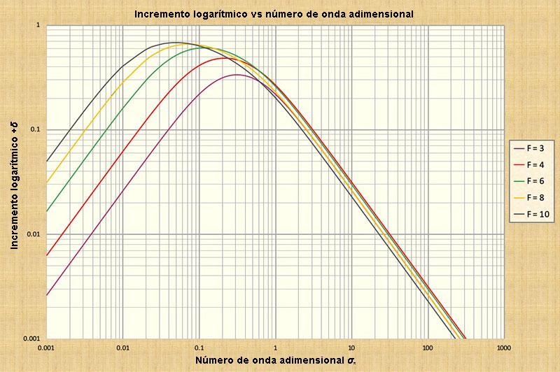
La cantidad de difusión se expresa en términos del decremento logarítmico δ, el cual mide la velocidad a la que la onda cambia durante la propagación (Wylie, 1966). La definición de decremento logarítmico es: δ = ln Q1 - ln Q0, o, alternativamente: Q1 = Q0 eδ, en la que Q0 = caudal de inundación al inicio de la medición, y Q1 = caudal de inundación después de un tiempo transcurrido igual a un período de propagación (sinusoidal). La descarga disminuye para un valor negativo de δ, provocando atenuación de la onda, correspondiente al número de Froude F < 2 (número de Vedernikov V < 1); aumenta para un valor positivo, es decir, un incremento logarítmico, provocando una amplificación de la onda, correspondiente al número de Froude F > 2 (V > 1) (Ponce, 1991). Ponce y Simons (1977). han utilizado la teoría de la estabilidad lineal para calcular el decremento logarítmico de la onda difusiva. La expresión es: δd = (2 π /3) σ*. Téngase en cuenta que en esta expresión, cuando σ* → 0, el decremento logarítmico δd → 0, lo que confirma que una onda cinemática no está sujeta a atenuación. Además, para σ* → ∞, el decremento logarítmico de la onda difusiva δd → ∞, lo que confirma la incapacidad de la fórmula de decremento logarítmico de la onda difusiva para tener en cuenta las ondas dinámicas, las cuales también presentan atenuación cero.
La Figura 2 muestra la variación del decremento logarítmico
para todos los tipos de onda, a través del rango de números
de onda adimensionales de 0,001 a 1000, para números de
Froude F < 2.
La Tabla 1 muestra los valores del decremento logarítmico de la onda de difusión δd relevantes en el contexto actual. El examen de este cuadro conduce a las conclusiones resumidas en el Cuadro A.
Confirmamos que las ondas cinemáticas no manifiestan atenuación. También confirmamos que, para el valor medio del número de onda adimensional σ* > 0,17, la atenuación de la onda es superior al 30%, un umbral que es considerado como el que marca la diferencia entre las ondas difusivas (cuya difusión es limitada, inferior al 30%) y las ondas mixtas (cuya difusión podría llegar el 100%) (Flood Studies Report, 1975). Por lo tanto, tiene sentido el argumento de que las ondas mixtas son muy disipativas y que, en la mayoría de los casos de interés práctico, probablemente no estén disponibles para su cálculo (Ponce, 1992). Confirmamos las siguientes observaciones, basadas en cálculos detallados, en referencia a la Fig. 1: (a) las ondas cinemáticas se ubican a lo largo del primer ciclo logarítmico, comenzando por la izquierda; (b) las ondas difusivas a lo largo del segundo y tercer ciclos; (c) las ondas mixtas a lo largo del cuarto y quinto ciclos; y (d) las ondas dinámicas a lo largo del quinto y sexto ciclos. Nótese que estas últimas dependen en gran medida del número de Froude. Las ondas cinemáticas no se atenúan, las ondas mixtas se atenúan considerablemente, y las ondas dinámicas, al ser característicamente cortas, no se asemejan a ondas de inundación, las cuales son característicamente largas. Por lo tanto, vemos que se justifica sólidamente la aplicabilidad de la onda difusiva para el cálculo del enrutamiento de inundaciones.
4. APLICABILIDAD DE LAS ONDAS DIFUSIVAS
.
Tras demostrar la aplicabilidad de las ondas de difusión al problema del enrutamiento de inundaciones, ahora demostramos su aplicabilidad. Aquí ahondamos en el trabajo de Ponce y otros (1978), quienes establecieron el criterio para la aplicabilidad de las ondas cinemáticas y difusivas en términos de las propiedades de las ondas de inundación.
Para el modelo de onda cinemática, Ponce y otros (1978) afirmaron que para lograr al menos un 95% de precisión de la solución de onda cinemática después de un período de propagación, el período adimensional debe satisfacer la siguiente desigualdad: Por ejemplo, dados los siguientes datos: uo = 3 pies/seg, do = 10 pies, y So = 0,0001, el período de onda resultante es: T > (171 × 10) / ( (0,0001 × 3) = 5.700.000 segundos = 65,97 días. En otras palabras, la duración de la inundación debe ser mayor que aproximadamente 66 días para que la solución de onda cinemática tenga una precisión de al menos el 95% después de un período de propagación. De ello se deduce que cuanto mayor sea la duración de la inundación, más cinemática será la onda de inundación; este hallazgo concuerda admirablemente con la teoría.
Para el modelo de onda de difusión, Ponce y otros (1978) compararon el decremento logarítmico
de la onda de difusión δd
con el de la solución completa (Fig. 2),
y concluyeron que para lograr al menos un 95% de precisión
de la solución de onda de difusión después de un período
de propagación, el período adimensional debe satisfacer
la siguiente desigualdad: τ* ≥ 30. En este caso,
el período adimensional se define de la siguiente manera:
5. UN EJEMPLO PRÁCTICO
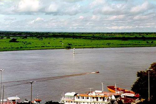
Los conceptos presentados en la sección anterior se aplican aquí a la cuenca
del río Alto Paraguay, en Mato Grosso do Sul, Brasil, y su vecina Bolivia. Este río presenta un entorno geográfico único, ya que fluye a través de un delta continental que comprende el Pantanal de Mato Grosso, considerado el humedal más grande del mundo, con una extensión de 136.700 km˛. El entorno geomorfológico,
hidrológico y ecológico de la cuenca del río Alto Paraguay ha sido descrito por Ponce (1995).
El hidrograma de crecida del río Alto Paraguay, en su tramo inferior, desde Ladario hasta Porto Murtinho, comprendiendo una distancia de 520 km a lo largo del río, presenta solamente un caudal pico, o máximo, condición atribuida a la extrema difusión del escurrimiento causada por la muy pequeńa pendiente del cauce del río, el cual varía entre 2,34 cm/km cerca de Ladario, y 0,83 cm/km cerca de Porto Murtinho, con un promedio de 1,6 cm/km.
Aguas abajo de Ladario, el nivel del río sube de marzo a agosto y baja de septiembre a febrero.
6. CONCLUSIONES
Se ha realizado una revisión de las ondas difusivas
y su uso para el enrutamiento de ondas de inundación.
Las ondas difusivas se propagan con la celeridad de Seddon,
es decir, la celeridad de la onda cinemática, y están sujetas
a poca atenuación (difusión). Estas propiedades coinciden
claramente con las de las ondas de inundación típicas.
Otras ondas de flujo en superficie libre, a saber,
las cinemáticas, mixtas y dinámicas, son ya sea no difusivas
(las cinemáticas y dinámicas) o demasiado difusivas (las mixtas).
En particular, se ha confirmado que las ondas mixtas son
tan difusivas que se puede cuestionar por completo su mera existencia.
Los criterios para la aplicabilidad de las ondas cinemáticas y
difusivas muestran que estas últimas, las ondas difusivas,
tienen un rango de aplicabilidad más amplio que el de las ondas
cinemáticas. Por lo tanto, se recomienda la onda difusiva
para aplicaciones prácticas en la hidrología de inundaciones.
Una aplicación con datos de campo en el Río Alto Paraguay,
en Mato Grosso do Sul, Brasil, confirma los hallazgos de este estudio.
REFERENCIAS
Lagrange, J. L. de. 1788. Mécanique Analytique, Paris, part 2, section II, article 2, 192.
Seddon, J. A. 1900.
River hydraulics. Transactions, ASCE, Vol.XLIII, 179-243, June.
Lighthill, M. J. y G. B. Whitham. 1955.
On kinematic waves. I. Flood movement in long rivers.
Proceedings,
Wylie, C. R. 1966. Advanced Engineering Mathematics, 3rd ed.,
McGraw-Hill Book Co., New York, NY.
Flood Studies Report. 1975. Vol. III: Flood Routing Studies,
Natural Environment Research Council, London, England.
Ponce, V. M. y D. B. Simons. 1977.
Propagación de ondas poco profundas en canales abiertos.
Journal of the Hydraulics Division, ASCE, 103(12), 1461-1476.
[Traducción al Español, 2021].
Ponce, V. M., R. M. Li, y D. B. Simons. 1978.
Aplicabilidad de los modelos de onda cinemática y difusiva.
Journal of the Hydraulics Division, ASCE, 104(3), 353-360.
[Traducción al Español, 2015].
Ponce, V. M. 1991.
Nueva perspectiva del número de Vedernikov.
Water Resources Research, Vol. 27, No. 7, 1777-1779, Julio.
[Traducción al Español, 2021].
Ponce, V. M. 1992.
Kinematic wave modeling: Where do we go from here?
International Symposium on Hydrology of Mountainous Areas, Shimla, India, May 28-30.
Ponce, V. M. 1995.
Hydrologic and environmental impact of the Parana-Paraguay waterway on the Pantanal of Mato Grosso, Brazil.
https://ponce.sdsu.edu/hydrologic_and_environmental_impact_of_the_parana_paraguay_waterway.html
Ponce, V. M. 2023.
Ondas cinemáticas y dinámicas: La declaración definitiva.
Online article. [Traducción al Español, 2025].
| ||||||||||||||||||||||||||||||||||||||||||||||||||||||||||||||||||||||||||||||||||||||||||||||||||||||


| 260124 |