|
|
| CHAPTER 1: INTRODUCTION |
1.1 OPEN-CHANNEL FLOW
|
|
Open-channel flow has a free surface and it is, therefore, subject to atmospheric pressure
|

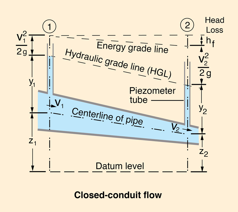
In closed-conduit flow, the cross section is fixed by the pipe boundaries. On the other hand, in open-channel flow, the flow cross section is not fixed, varying with the flow. In closed-conduit flow, the roughness varies from smooth brass to corroded pipes; in open-channel flow, it varies from acrylic glass or lucite® (a very smooth type of plastic), to that of natural stream channels and their neighboring flood plains.
In closed-conduit flow, the
hydraulic pressure at the center of the pipe defines the hydraulic grade line (HGL in Fig. 1-2).
The hydraulic pressure (head of water) above the centerline of the pipe is referred to as the piezometric head.
The energy grade line includes the velocity head
|
In open-channel flow, the flow depth measured above the
channel bottom defines the water surface elevation,
which is equivalent to the hydraulic grade line of closed-conduit flow; see Fig. 1-3.
The total energy grade line includes the velocity head
|
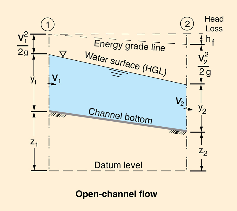
Note the difference between closed-conduit and open-channel flow. In closed-conduit flow, water will rise in a piezometer tube up the level where it defines the hydraulic grade line associated with the hydraulic pressure in the conduit. On the other hand, in open-channel flow, the water surface is the hydraulic grade line, which is at atmospheric pressure.
1.2 TYPES OF FLOW
|
|
There are two general types of open-channel cross sections:
- Prismatic, and
- Nonprismatic.
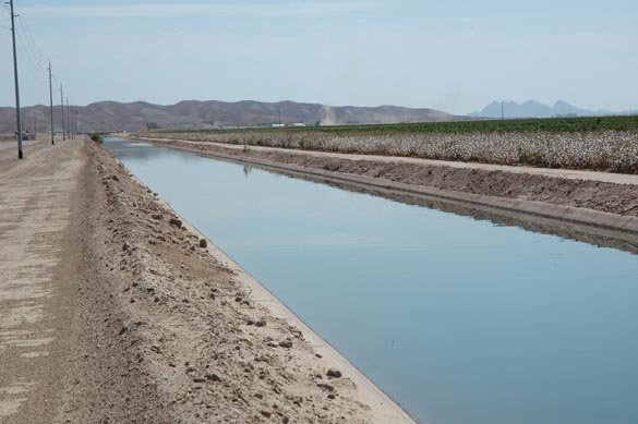
Artificial, or human-made channels, are usually prismatic, featuring a constant shape and size, at least for a certain length of channel. Conversely, natural channels are typically nonprismatic, i.e., the shape and size of the cross section varies along the channel. Artificial channels are also referred to as canals.
Several geometric and hydraulic properties help describe an open channel (Fig. 1-4). These are:
- Discharge Q,
- Flow area A,
- Mean velocity V, with V = Q /A,
- Wetted perimeter P,
- Top width T,
- Hydraulic radius R, with R = A /P,
- Hydraulic depth D, with D = A /T,
- Channel width B,
- Channel bottom elevation, or bed elevation z,
- Flow depth d,
- Stage, or water surface elevation, with y = z + d.
|
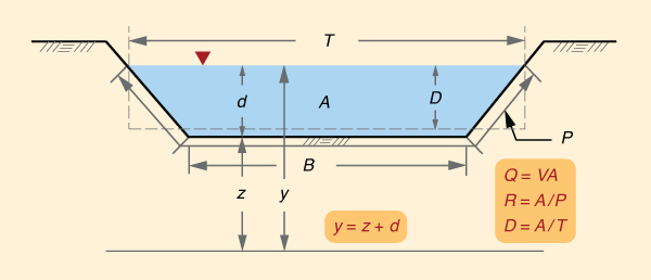
In prismatic channels, the flow depth d is often referred to as y, particularly when it cannot be confused with stage. Also, the channel side slope is often referred to as z H : 1 V, particularly when it cannot be confused with bed elevation.
Classification of open-channel flow
Open-channel flow may be classified as follows:
- Steady or unsteady.
- Uniform or equilibrium.
- Gradually varied or rapidly varied.
- Spatially varied.
The flow is steady when the hydraulic variables (discharge, flow area, mean velocity, flow depth, and so on) do not vary in time. Conversely, the flow is unsteady when the hydraulic variables vary in time and space. Steady flow is relatively simple to calculate, compared to unsteady flow.
The flow is uniform when the channel is prismatic and the hydraulic variables (Q, A, V, d, and so on) are constant in time and space. The flow is in equilibrium when the channel is nonprismatic and the hydraulic variables are approximately constant in time and space. The calculation of uniform flow is relatively straight forward when compared to that of other states of flow.
The flow is gradually varied when the discharge Q is constant but the other hydraulic variables (A, V, d, and so on) vary gradually in space. Under gradually varied flow, the pressure distribution in the vertical direction, normal to the flow, is very close to hydrostatic, i.e., proportional to the flow depth.
The flow is rapidly varied when the discharge is constant but the other hydraulic variables (A, V, d, and so on) vary rapidly in space, in such a way that a hydrostatic pressure distribution cannot be assumed in the vertical direction normal to the flow. While the calculation of gradually varied flow is somewhat involved but doable, the calculation of rapidly varied flow is generally more complex, in practice being based on empirical formulas, for lack of a theoretical solution.
The flow is spatially varied when the discharge Q varies in space only, i.e., along the channel, typically due to lateral inflow or outflow.
Occurrence of various types of flow
Steady uniform flow occurs in a prismatic channel (Fig. 1-5); steady equilibrium flow occurs in a nonprismatic channel. Unsteady uniform flow does not exist in nature, because the flow cannot be uniform and unsteady at the same time. The word "unsteady" implies nonequilibrium; thus, unsteady equilibrium flow does not exist.
|
Steady gradually varied flow is represented by the water surface profiles, also referred to as backwater (or drawdown) computations (Chapter 7). Unsteady gradually varied flow is the calculation of flood flows, or flood routing (Chapter 10).
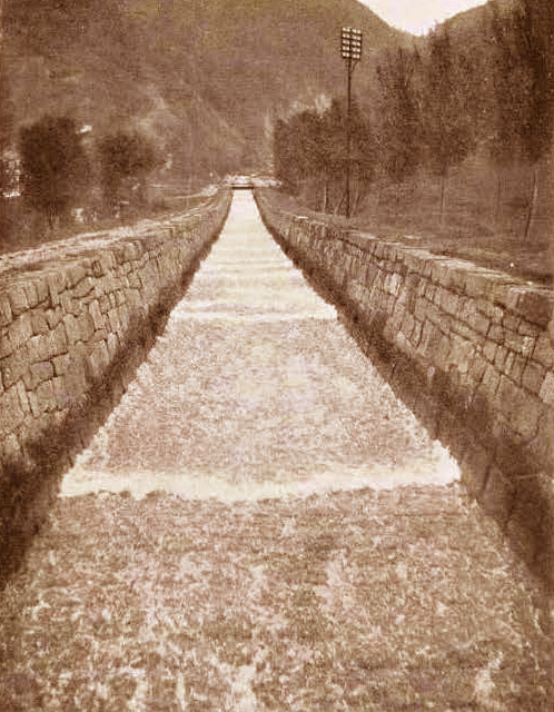
Steady rapidly varied flow is represented by the flow over spillways or the hydraulic jump. Unsteady rapidly varied flow is represented by the moving hydraulic jump, surges, roll waves, kinematic shocks, and tidal bores. Figure 1-6 shows a train of roll waves in a steep irrigation canal.
Spatially varied flow occurs in an artificial canal when the discharge is varying along the channel, due to lateral water extractions or channel overflow.
|
1.3 STATE OF FLOW
|
|
The state of open-channel flow may be described in terms of certain characteristic velocities and
viscosities.
Velocity is the ratio of length (distance) over time, with units
Velocity ratios
There are three characteristic velocities in open-channel flow:
The mean velocity u of the steady uniform flow;
The velocity, or celerity ck of kinematic waves; and
The velocity, or celerity (actually, two celerities) cd of dynamic waves.
The mean velocity of the steady uniform flow using the Manning equation (SI units) is:
|
1 u = _____ R 2/3 S 1/2 n | (1-1) |
in which n = Manning's friction coefficient, R = hydraulic radius, and S = friction slope.
The mean velocity of the steady uniform flow using the Chezy equation is:
|
u = C R 1/2 S 1/2 | (1-2) |
in which C = Chezy friction coefficient.
In general, four forces are active in a control volume in open-channel flow. These forces are due to friction, gravity, the pressure (flow depth) gradient, and inertia. Kinematic waves are those where the momentum balance is expressed in terms of the frictional and gravitational forces only (Lighthill and Whitham, 1955).
The celerity of kinematic waves, or Seddon celerity, is (Seddon, 1900; Chow, 1959; Ponce, 1989):
|
ck = β u | (1-3) |
in which β = exponent of the discharge-flow area rating, defined as follows:
|
Q = α Aβ | (1-4) |
Dynamic waves are those where the momentum balance is expressed in terms of the pressure-gradient and inertial forces only. The celerity of dynamic waves is:
|
cd = u ± (g D )1/2 | (1-5) |
in which g = gravitational acceleration, and D = hydraulic depth, D = A /T.
From Eq. 1-3, the relative celerity of kinematic waves is:
|
v = (β - 1) u | (1-6) |
From Eq. 1-5, the (absolute value of the) relative celerity of dynamic waves is:
|
w = (g D )1/2 | (1-7) |
For rectangular channels, for which D = d, or for hydraulically wide channels, for which D ≅ d, the relative celerity of dynamic waves is:
|
w = (g d )1/2 | (1-8) |
Equation 1-8 is known as the Lagrange (relative) celerity equation, after Lagrange (1788), who first derived it.
The Froude Number
The Froude number is defined as follows (Chow, 1959):
|
u F = _____ w | (1-9) |
The Froude number characterizes the condition of:
- F < 1: Subcritical flow, or u < w,
- F = 1: Critical flow, or u = w,
- F > 1: Supercritical flow, or u > w.
Under subcritical flow, surface waves (perturbations) can travel upstream, because their upstream celerity -w is greater than the mean flow velocity u.
Under critical flow, surface waves (perturbations) remain stationary, because their (absolute) celerity w is equal to the mean flow velocity u.
Under supercritical flow, surface waves (perturbations) can travel downstream only, because their upstream celerity -w is smaller than the mean flow velocity u.
The Vedernikov Number
The Vedernikov number is defined as follows (Vedernikov, 1945; 1946; Powell, 1948; Craya, 1952):
|
v V = _____ w | (1-10) |
The Vedernikov number characterizes the following states of flow:
- V < 1: Stable flow, or v < w,
- V = 1: Neutrally stable flow, or v = w,
- V > 1: Unstable flow, or v > w.
Under stable flow, the relative kinematic wave celerity v is smaller than the relative dynamic wave celerity w and, therefore, surface waves (perturbations) are able to attenuate (dissipate).
Under neutrally stable flow, the relative kinematic wave celerity v is equal to the relative dynamic wave celerity w and, therefore, surface waves (perturbations) neither attenuate nor amplify. Amplification amounts to negative dissipation.
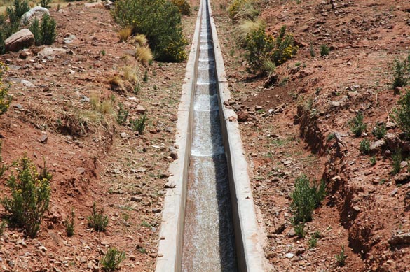
Under unstable flow, the relative kinematic wave celerity v is greater than the relative dynamic wave celerity w. Therefore, surface waves (perturbations) are subject to amplification. In practice, the condition V ≥ 1 leads to the development of roll waves, a train of waves that travel downstream, typically in artificial channels of steep slope (Cornish, 1907) (Fig. 1-7).
|
| ||||
|
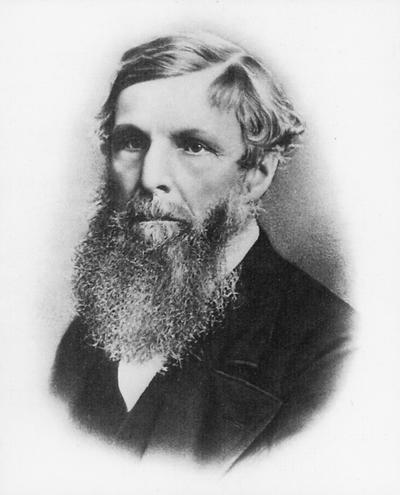
William Froude was born in Dartington, Devon, England on November 28, 1810 and died
from a stroke on a cruise to Simonstown, South Africa at age 69. He was an engineer,
hydrodynamicist and naval architect.
He acquired his education in mathematics at Oxford in 1832. Immediately after
his graduation, he worked for Isambard Kingdom Burnel, the famed developer of railways, as a surveyor on the Great Western Railway,
in England.
In 1857, Brunel consulted him
on the behavior of the Great Eastern ship at sea. Based on Froude's recommendations,
Brunel modified the design of the ship to avoid rolling.
Starting in 1859, Froude built the first towing tank, using his own resources.
He carried out ship model experiments using the tank,
first at his home in Paignton, and
later, in his other home, called Chelston Cross, in Torquay.
In 1861, he wrote a paper on the design of ship stability in a seaway.
The paper was published in the Proceedings of the Institution of Naval Architects. Later, between 1863 and 1867, he showed
that scaling between model and prototype (the actual ship) applied (i.e., the frictional resistance was equal)
when the speed (V) was proportional to the square root of the length (L).
He called this concept the "Law of Comparison."
V = k (L)1/2
in which k is the number that applies to both model and prototype.
This law is known as Froude's law, even though Froude himself recognized that
Ferdinand Reech (1805-1850) had presented the concept twenty
years earlier.
Froude's work was pioneering because he was the first to identify
the most efficient shape for the hull of ships,
as well as to predict ship stability with reference to reduced-scale models.
In open-channel hydraulics, Froude's Law is embodied in the Froude number, defined as:
F = V / (gD) 1/2
in which V = mean velocity, D = hydraulic depth, and g = gravitational acceleration.
Unlike Froude's original relation (k), the Froude number F is dimensionless.
The L has been replaced by D to better represent the force of gravity in open-channel flow.
|
The exponent β
of the discharge-area rating
The three velocities u, v, and w lead to only two independent velocity ratios, the Froude (Eq. 1-8) and Vedernikov (Eq. 1-9) numbers. The third ratio:
|
v
V β - 1 = _____ = _____ u F | (1-11) |
is the dimensionless relative kinematic wave celerity, equal to the exponent of the discharge-area rating minus 1. Thus, it is seen that the exponent β in Eq. 1-4 is a function of both the Froude and Vedernikov numbers.
The value of β varies with the type of friction regime (laminar, transitional, or turbulent; and turbulent Manning or Chezy) and cross-sectional shape. For laminar flow, β = 3. For turbulent flow, under Manning friction: 1 ≤ β ≤ 5/3, depending on the shape of the cross section. For turbulent flow, under Chezy friction: 1 ≤ β ≤ 3/2, depending on the shape of the cross section.
Types of cross-sectional shape
There are three asymptotic cross-sectional shapes in open channels:
The hydraulically wide channel, for which the wetted perimeter P is a constant (Ponce and Porras, 1995). In this case,
β = 5/3 for Manning friction and β = 3/2 for Chezy friction. Generally, a channel cross-section is considered to be hydraulically wide for values of the ratio of top width to flow depthT /d > 10. In practice, most natural channels are hydraulically wide (Fig. 1-8).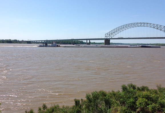
Nuccitelli Fig. 1-8 Mississippi river at Mud Island, Memphis, Tennessee.
The triangular channel, in which the top width T is proportional to the flow depth d (Fig. 1-9). In this case,
β = 4/3 for Manning friction and β = 5/4 for Chezy friction. Roadside drainage (gutters) often feature a triangular cross section.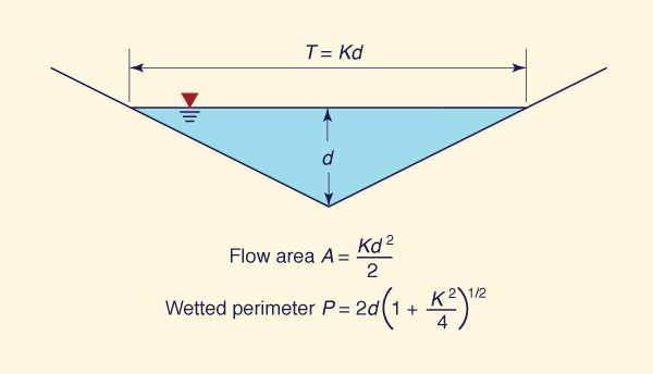
Fig. 1-9 The triangular cross section.
The inherently stable channel (Fig. 1-10), for which the hydraulic radius R, corresponding to the maximum depth in the lower subsection, is constant in the upper subsection (Ponce and Porras, 1995). The lower subsection is required to provide a finite value of R applicable to the upper subsection. The value of β ≡ 1 in the upper subsection.
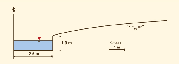
Fig. 1-10 The inherently stable channel.
Neutrally stable flow
For neutral stability: V = 1. Therefore, from Eq. 1-11, the Froude number corresponding to neutrally stable flow is:
|
1 Fns = ________ β - 1 | (1-12) |
Table 1-1 shows values of Fns for selected values of β. It is seen that as β varies from β = 3 (laminar flow) to β = 1 (inherently stable channel), the value of Fns varies from Fns = 1/2 to Fns = ∞. In other words, as β ⇒ 1, Fns ⇒ ∞.
In practice, since friction has effectively a lower bound, the Froude number is restricted to an upper bound, which is seldom likely to exceed F = 25. Therefore, in most cases, a value of β = 1.04 would be already stable for practical purposes.
| Table 1-1 Values of Fns for selected values of β. | |||
| β | Type of friction | Shape of cross section | Fns |
| 3 | Laminar | Hydraulically wide | 1/2 |
| 8/3 | Mixed laminar-turbulent (25% turbulent Manning) |
Hydraulically wide | 3/5 |
| 21/8 | Mixed laminar-turbulent (25% turbulent Chezy) |
Hydraulically wide | 8/13 |
| 7/3 | Mixed laminar-turbulent (50% turbulent Manning) |
Hydraulically wide | 3/4 |
| 9/4 | Mixed laminar-turbulent (50% turbulent Chezy) |
Hydraulically wide | 4/5 |
| 2 | Mixed laminar-turbulent (75% turbulent Manning) |
Hydraulically wide | 1 |
| 15/8 | Mixed laminar-turbulent (75% turbulent Chezy) |
Hydraulically wide | 8/7 |
| 5/3 | Turbulent Manning | Hydraulically wide | 3/2 |
| 3/2 | Turbulent Chezy | Hydraulically wide | 2 |
| 4/3 | Turbulent Manning | Triangular | 3 |
| 5/4 | Turbulent Chezy | Triangular | 4 |
| 1 | Any | Inherently stable | ∞ |
As shown in Table 1-1, values of β in open-channel
and overland flow are limited in the range
Viscosity ratios
There are three characteristic viscosities in open-channel flow:
The internal viscosity, or kinematic viscosity ν of the fluid (Appendix A),
The external viscosity (or hydraulic diffusivity νh) of the steady flow; and
The external viscosity (or wave diffusivity νw) of the unsteady flow.
The kinematic viscosity ν of the fluid varies as a function of temperature (Appendix A).
The concept of hydraulic diffusivity νh is due to Hayami (1951). Hayami combined the governing equations of open-channel flow (Chapter 10) to develop a single convection-diffusion equation, i.e., an equation describing the convection (first-order process) and diffusion (second-order process) of a flood wave. The hydraulic diffusivity is defined as follows:
|
qo νh = _______ 2 So | (1-13) |
in which qo = equilibrium unit-width discharge, and So = friction (energy) slope. It is seen that flood wave diffusion is directly proportional to unit-width discharge and inversely proportional to friction (energy) slope.
Equation 1-13 can be expressed in terms of velocity and flow depth as follows:
|
uo do νh = _________ 2 So | (1-14) |
A related value of diffusivity, which is independent of slope, is:
|
νh' = uo do | (1-15) |
In general, for an arbitrary cross-sectional shape:
|
νh' = uo Ro | (1-16) |
in which Ro = hydraulic radius.
In kinematic wave theory, the characteristic reach length is defined as follows (Lighthill and Whitham, 1955):
|
do Lo = ______ So | (1-17) |
in which Lo is the length of channel in which the equilibrium flow drops a head equal to its depth. Thus, in terms of the characteristic reach length, the hydraulic diffusivity is:
|
uo Lo νh = _______ 2 | (1-18) |
In a manner resembling the hydraulic diffusivity, the wave diffusivity is conveniently defined as follows:
|
uo L νw = _______ 4 π | (1-19) |
in which L = wavelength of the disturbance.
The Reynolds Number
The Reynolds number R is (Chow, 1959):
|
vh' uo Ro R = ______ = ________ ν ν | (1-20) |
The Reynolds number R describes the flow regime as either:
- Laminar,
- Transitional, or
- Turbulent.
Under steady flow conditions in open-channel flow, laminar flow occurs for R ≤ 500 and turbulent flow for R > 2000. Transitional flow occurs in the intermediate range: 500 < R ≤ 2000. Under unsteady flow, the mixed laminar-turbulent flow described in Table 1-1 is akin to transitional flow, featuring a comparable range of Reynolds numbers.
In practice, most open-channel flow cases are in the turbulent regime. Conversely, most overland flow cases (i.e., free-surface plane flow) are in the laminar or mixed laminar-turbulent regime.
The dimensionless wavenumber
The dimensionless wavenumber σ is defined as follows (Ponce and Simons, 1977):
|
νh 2 π σ = ______ = _____ Lo νw L | (1-21) |
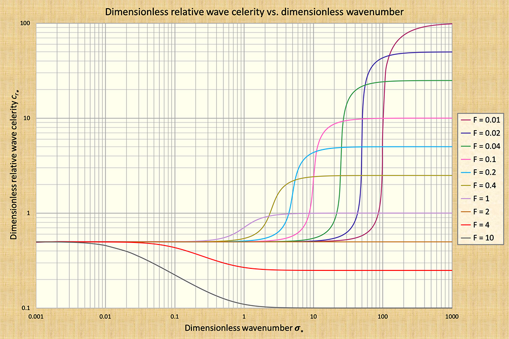
The wavenumber σ describes the dimensionless length scale of the wave, as shown in Fig. 1-11, in terms of: (a) kinematic waves, (b) dynamic waves, and (c) mixed kinematic-dynamic waves. Figure 11 is applicable for the case of Chezy friction in hydraulically wide channels.
Under kinematic flow, depicted on the left side of Fig. 1-11:
The momentum balance is described only in terms of the frictional and gravitational forces,
The dimensionless relative kinematic wave celerity (Eq. 1-3), a constant for all wavenumbers and Froude numbers, prevails, and
Wave attenuation is theoretically zero.
Under dynamic flow, depicted on the right side of Fig. 1-11:
The momentum balance is described only in terms of the pressure-gradient and inertial forces,
The dimensionless relative dynamic wave celerity (Eq. 1-5), a constant for all wavenumbers and varying with Froude number, prevails, and
Wave attenuation is theoretically zero.
Under mixed kinematic-dynamic flow, depicted by the middle section of Fig. 1-11:
The momentum balance incorporates all four forces present in unsteady open-channel flow (frictional, gravitational, pressure-gradient, and inertial),
There is no characteristic celerity and, therefore, the wave is subject to very strong attenuation in the midrange of dimensionless wavenumbers,
For each curve depicted in Fig. 1-11, the attenuation rate is a maximum at the point of inflexion (See Chapter 10) (Ponce and Simons, 1977).
|
Dynamic hydraulic diffusivity
The dynamic hydraulic diffusivity, which unlike the Hayami hydraulic diffusivity of
|
uo Lo νh = _______ (1 - V 2) 2 | (1-22) |
For low Vedernikov numbers, V ⇒ 0, the dynamic hydraulic diffusivity reduces to the expression for kinematic hydraulic diffusivity, i.e., Eq. 1-18. Conversely, for high Vedernikov numbers, V ⇒ 1, and the dynamic hydraulic diffusivity vanishes. Under this flow condition, the total absence of wave attenuation is conducive to the development of roll waves (Figs. 1-6 and 1-7).
|
A word of caution regarding the usage of the term "dynamic wave"
In hydraulic engineering practice, the mixed kinematic-dynamic wave,
which includes all the terms in the momentum equation--friction, gravity, pressure gradient, and inertia--is commonly
referred to as "dynamic wave," following the work of Fread (1993).
However, the original dynamic wave
of Lagrange (1788) accounted only for pressure gradient and inertia.
To add to the confusion, the dynamic wave of Lagrange has often been referred
to as "gravity wave." Clearly, the term "gravity wave" is not appropriate,
because the gravity force is ostensibly missing from its formulation.
Thus, it appears better to reserve the term "kinematic" for waves governed by friction and gravity (following
Lighthill and Whitham), "dynamic"
for waves governed by pressure gradient and inertia (following Lagrange),
and to use "mixed kinematic-dynamic" for waves
governed by the complete momentum statement (all four forces). |
1.4 FLOW REGIMES
|
|
The flow regimes in open-channel flow are:
- Laminar,
- Transitional, and
- Turbulent.
The flow regimes are characterized by the Reynolds number R, Eq. 1-20. In open-channel flow, the laminar regime prevails for R ≤ 500, the transitional regime for 500 < R ≤ 2000, and the turbulent regime for R > 2000.
The flow regimes vary with roughness of the channel surface. Figure 1-12 shows the relation between Reynolds number R and Darcy-Weisbach friction factor f for flow in smooth channels. Figure 1-13 shows the relation between Reynolds number R and Darcy-Weisbach friction factor f for flow in rough channels.
The Darcy-Weisbach friction formula, developed in connection with flow in pipes, is:
|
L
V 2 hf = f _____ ______ do 2 g | (1-23) |
in which hf = frictional head loss; f = Darcy-Weisbach friction factor; L = length of the pipe; do = pipe diameter; V = mean flow velocity in the pipe; and g = gravitational acceleration.
|

|

The examination of Figs. 1-12 and 1-13 enables the following conclusions:
Laminar flow prevails under low Reynolds numbers. Under laminar flow, the Darcy-Weisbach friction factor is inversely proportional to the Reynolds number. In general:
K
f = _____
R(1-24) in which K is a constant varying between 14 (for triangular channels) and 24 (for rectangular channels) for smooth channel surfaces, and between 33 and 60 for rough channel surfaces.
The transitional range is not well defined, depending to some extent on channel shape. For practical purposes, the transitional range for open-channel flow may be assumed to be:
500 ≤ R ≤ 2000. Under turbulent flow, the relation between f and R follows the Blasius formula (Chow, 1959):
0.223
f = _________
R 0.25(1-25) This equation is valid for Reynolds numbers in the range: 750 ≤ R ≤ 25,000.
A general expression for the relation between f and R was developed by von Karman and later modified by Prandlt to agree more closely with the applicable data. The resulting Prandtl-von Karman equation is (Chow, 1959):
1
_______ = 2 log (R f 1/2 ) + 0.4
f 1/2(1-26)
Note that the Prandtl-von Karman equation can be expressed in explicit form as follows:
|
1 R = _______ 10 [ ( 1 - 0.4 f 1/2 ) / ( 2 f 1/2 ) ] f 1/2 | (1-27) |
The Darcy-Weisbach friction factor for open-channel flow
The Darcy-Weisbach formula, Eq. 1-23, is strictly applicable to closed-conduit (pipe) flow. In pipe flow, the characteristic frictional length is the pipe diameter do. On the other hand, in open-channel flow, the characteristic frictional length is the hydraulic radius R, i.e., the ratio of flow area to wetted perimeter:
|
A R = ______ P | (1-28) |
Since the flow area of a circular pipe (flowing full) is A = π do2/4, and the wetted perimeter is
|
L
V 2 hf = f ______ ______ 4R 2g | (1-29) |
in which V = mean flow velocity in the channel.
In open-channel flow, the energy slope, which under steady flow is the same as friction, bed, or bottom slope, is:
|
hf
V 2 f V 2 S = ______ = f _______ = ___ _______ L 8gR 8 gR | (1-30) |
For any arbitrary cross-sectional shape, the Froude number is:
|
V F = __________ (gD)1/2 | (1-31) |
in which D = hydraulic depth: D = A /T.
Equation 1-30 can be expressed in terms of the Froude number as follows:
|
f D S = ___ _____ F 2 8 R | (1-32) |
Equation 1-32 states the proportionality between energy slope and Froude number, with the proportionality factor being a function of the Darcy-Weisbach friction factor and the shape factor D /R.
For a hydraulically wide channel, for which D ≅ R, Eq. 1-32 reduces to:
|
f S = ___ F 2 8 | (1-33) |
Thus, for a hydraulically wide channel, the proportionality factor between energy slope and Froude number is only a function of the Darcy-Weisbach friction factor. In essence, for application to open-channel flow, a modified Darcy-Weisbach friction factor f, equal to 1/8 of the conventional Darcy-Weisbach friction factor f is applicable. The modified Darcy-Weisbach equation for open-channel flow is:
|
S = f F 2 | (1-34) |
Table 1-2 shows approximate values of Darcy-Weisbach friction factor f and corresponding modified friction factor f for selected values of R in the turbulent range.
| Table 1-2 Approximate values of friction factors
f and f for selected values of R in the turbulent range. |
||
| R | f | f |
| 2000 | 0.036 | 0.0045 |
| 4000 | 0.032 | 0.004 |
| 7000 | 0.028 | 0.0035 |
| 10000 | 0.024 | 0.003 |
| 15000 | 0.020 | 0.0025 |
| 60000 | 0.016 | 0.002 |
|
On the proportionality between energy slope and Froude number
Equation 1-33 reveals a fundamental property of open-channel flow in the turbulent range: The proportionality between energy slope and Froude number.
The following relations hold:
For
f constant, the energy
slope S will increase proportionally with an increase in Froude number
F, and vice versa.
For
F constant, the energy slope S
will increase proportionally with an increase in friction factor f, and vice versa.
For S constant,
the Froude number F
will increase proportionally with a decrease in friction factor f, and vice versa.
|
QUESTIONS
|
|
What is the difference between flow depth d and hydraulic depth D?
Is unsteady uniform flow possible? Why not?
What four forces are acting in the momentum balance in open-channel flow?
What is a kinematic wave?
What is a dynamic wave according to Lagrange?
What is the Froude number?
What is the Vedernikov number?
What is neutrally stable flow?
What is the normal range in the exponent β of the discharge-flow area rating in open-channel and free-surface flow?
What type of friction is described by β = 2?
For what condition can the value of β be less than 1?
What is the Reynolds number?
What is the commonly estimated range of Reynolds numbers for the transitional regime in open-channel flow?
What is the dimensionless wavenumber?
Do kinematic waves attenuate?
Do dynamic waves attenuate?
Do mixed kinematic-dynamic waves attenuate?
Which type of open-channel flow wave attenuates the most?
For what value of dimensionless wavenumber is the attenuation rate of mixed kinematic-dynamic waves a maximum?
What is the dimensionless relative kinematic wave celerity under Chezy friction for a hydraulically wide channel?
What is the characteristic reach length?
What is the hydraulic diffusivity?
For what value of channel slope is the hydraulic diffusivity a maximum?
What is the dynamic hydraulic diffusivity?
Under what flow condition does the dynamic hydraulic diffusivity vanish?
In hydraulic engineering practice, what does the term "dynamic wave" commonly refer to?
What is the modified Darcy-Weisbach formula, applicable to open-channel flow?
What is the typical range of Darcy-Weisbach friction factor f in the turbulent range?
What is the typical range of the modified Darcy-Weisbach friction factor f in the turbulent range?
Is there a theoretical upper limit to the Froude number? How can it be calculated?
PROBLEMS
|
|
Derive the expression for the angle θ in a circular channel (culvert) as a function of flow depth y and diameter D, where D = 2r (Fig. 1-14).
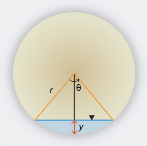
Fig. 1-14 Definition sketch for a circular channel.
Show that the maximum discharge in a circular channel (Fig. 1-14) is attained at y = 0.94 D. Use ONLINE CHANNEL 03. Explain the reason for this behavior.
Derive the formula for flow area A, wetted perimeter P, and top width T for a trapezoidal channel, in terms of flow depth y, bottom width b and side slope z H: 1 V (Fig. 1-15).

Fig. 1-15 Definition sketch for a trapezoidal channel.
Assume a trapezoidal channel of flow depth y, bottom width b, and side slope z H: 1 V
(Fig. 1-15). For a given z, derive an expression for the width-to-depth ratio b/y as a function of α, the ratio of hydraulic depth D to flow depth y . With z = 1 and α = 0.99, what is the value of b/y?Calculate the dimensionless relative kinematic wave celerity under Manning friction for a hydraulically wide channel.
What is the value of β for a hydraulically wide channel at Froude number
F = 1.8 and Vedernikov number V = 0.9?A hydraulically wide channel has flow depth = 1 m, and flow velocity = 1.5 m/s. Calculate the Froude number. Confirm with ONLINE FROUDE.
A hydraulically wide channel has an exponent of the rating β = 1.6. The flow depth is 1 m, and the flow velocity 1.5 m/s. Calculate the Vedernikov number. Confirm with ONLINE VEDERNIKOV.
Given a hydraulically wide channel with Manning friction, and mean velocity u = 1 m/s, flow depth d = 1 m, and bottom slope S = 0.001. Determine the kinematic and dynamic hydraulic diffusivities.
Given a hydraulically wide channel with Chezy friction, and flow depth d = 1 m. What mean velocity will make the dynamic hydraulic diffusivity vanish?
According to the Blasius formula, what is the Reynolds number R corresponding to a Darcy-Weisbach friction factor f = 0.03?
According to the Prandt-von Karman formula, what is the Reynolds number R corresponding to a Darcy-Weisbach friction factor f = 0.03?
A WES spillway downstream slope is 0.6 H to 1 V. The Darcy-Weisbach friction factor is
f = 0.03. Calculate the maximum possible Froude number for these conditions.Assuming a maximum possible Froude number F = 25, calculate the value of β that will assure neutrally stable flow.
A prismatic channel is flowing close to critical flow. The bottom slope is S = 0.004. What is the value of the Darcy-Weisbach's modified friction factor f?
REFERENCES
|
|
Chow, V. T. 1959. Open-channel Hydraulics. Mc-Graw Hill, New York.
Cornish, V. 1907. Progressive waves in rivers. The Geographical Journal. Vol. 29, No. 1, January, 23-31.
Craya, A. 1952. The criterion for the possibility of roll wave formation. Gravity Waves, Circular 521, 141-151, National Institute of Standards and Technology, Gaithersburg, Md.
Dooge, J. C. I., W. B. Strupczewski, and J. J. Napiorkoswki. 1982. Hydrodynamic derivation of storage parameters in the Muskingum model. Journal of Hydrology, 54, 371-387.
Fread, D. 1993. "Flow Routing," Chapter 10 in Handbook of Hydrology, D. R. Maidment, editor, McGraw-Hill, New York.
Hayami, I. 1951. On the propagation of flood waves. Bulletin, Disaster Prevention Research Institute, No. 1, December.
Lagrange, J. L. de. 1788. Mécanique analytique, Paris, part 2, section II, article 2, p 192.
Lighthill, M. J., and G. B. Whitham. 1955. On kinematic waves: I. Flood movement in long rivers. Proceedings, Royal Society of London, Series A, 229, 281-316.
Ponce, V, M., and D. B. Simons. 1977. Shallow wave propagation in open-channel flow. Journal of the Hydraulics Division, ASCE, Vol. 103, No. HY12, December, 1461-1476.
Ponce, V. M. 1989. Engineering Hydrology: Principles and Practices. Prentice-Hall, Englewood Cliffs, New Jersey.
Ponce, V. M. 1991a. The kinematic wave controversy. Journal of Hydraulic Engineering, ASCE, Vol. 117, No. 4, April, 511-525.
Ponce, V. M. 1991b. New perspective on the Vedernikov number. Water Resources Research, Vol. 27, No. 7, 1777-1779, July.
Ponce, V. M., and P. J. Porras. 1995. Effect of cross-sectional shape on free-surface instability. Journal of Hydraulic Engineering, ASCE, Vol. 121, No. 4, April, 376-380.
Powell, R. W. 1948. Vedernikov's criterion for ultra-rapid flow. Transactions, American Geophysical Union, Vol. 29, No. 6, 882-886.
Seddon, J. A. 1900. River hydraulics. Transactions, ASCE, Vol. XLIII, 179-243, June.
Vedernikov, V. V. 1945. Conditions at the front of a translation wave disturbing a steady motion of a real fluid, Dokl. Akad. Nauk USSR, 48(4), 239-242.
Vedernikov, V. V. 1946. Characteristic features of a liquid flow in an open channel, Dokl. Akad. Nauk USSR, 52(3), 207-210.
| http://openchannelhydraulics.sdsu.edu |
|
210212 05:05 |