|
ABSTRACT
The inherently stable channel and its conditionally stable
alternative are reviewed, elucidated, and
calculated online.
The asymptotic neutrally stable Froude number for the inherently stable channel
is Fns ⇒ ∞.
Theoretically, such a channel will become neutrally stable when the Froude number reaches infinity.
Since the latter is a physical impossibility,
this requirement effectively guarantees that
the inherently stable channel will always remain well
below the threshold of instability, regardless of flow discharge,
thus completely eliminating the possibility of roll wave formation.
The inherently stable channel will never achieve
the value of Froude number Fns = ∞ which characterizes it.
Therefore, constructing an inherently stable channel provides an unrealistically high factor of safety against roll waves.
This suggests the possibility of designing instead a conditionally stable cross-sectional shape, for a suitably high but realistic
Froude number such as Fns = 25,
for which the risk of roll waves
would be so small as to be of no practical concern.
|
1. INTRODUCTION
The inherently stable channel is that for which
the asymptotic neutrally stable Froude number reaches infinity
(Fns ⇒ ∞)
(Ponce and Porras, 1993a).
Theoretically, such a channel will become neutrally stable, i.e.,
with Vedernikov number V = 1, when the Froude number reaches infinity
(F ⇒ ∞). Since the latter is a physical impossibility,
this requirement effectively guarantees that
the inherently stable channel will always remain well
below the threshold V = 1, regardless of flow discharge,
thus eliminating the possibility of roll wave formation.
As its name implies, an inherently stable channel is, by definition, unconditionally stable.
In a seminal paper on hydrodynamic stability,
Liggett (1975) noted that the theory of the inherently stable channel had not been experimentally verified. To the authors' knowledge, the inherently stable channel has never been built.
Yet, theory tells us that it may be an effective way of avoiding roll waves in steep open channels.
In certain hilly geomorphological settings, urban drainage may
often demand the
construction of large steep channels. As these channels reach flood stage,
the risk is high that the flow will become unstable at some point.
The
following video shows a telling story of the risk of channel instability in steep urban channels.
|
Watch video of pulsating waves in
La Paz, Bolivia
on February 24, 2016, at 05:30 pm. |
The recurrence of these pulsating waves in channelized rivers of the La Paz region has been documented by Molina et al. (1995).
In this article, we review the theory of the inherently stable channel, clarify its physical and
mathematical basis,
and develop an online calculator. It is hoped that this contribution will encourage the
hydraulic engineering profession to
try the inherently stable channel to avoid the risk of roll waves in steep urban channels.
2. THEORETICAL BACKGROUND
The criterion for the instability of open-channel flow is due to Vedernikov (1945, 1946).
Powell (1948)
gave this criterion the name of Vedernikov number.
Subsequently, Craya (1952) clarified the concept, enhancing its theoretical basis. The Vedernikov criterion
states that the water surface of a steep open channel
may become unstable, with the possibility of developing roll waves,
when the relative kinematic wave celerity, i.e., the Seddon celerity (Seddon, 1900), equals or exceeds the
relative dynamic wave
celerity, or Lagrange celerity (Lagrange, 1788).
In their
comprehensive study of shallow wave propagation in open-channel flow,
Ponce and Simons (1977) confirmed the validity of the Vedernikov criterion,
which for the case of Chezy friction is equivalent to Froude number F ≥ 2.
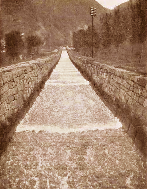
Roll waves are a train of waves occurring in steep channels of rigid boundary,
lined with either masonry or concrete. Figure 1 shows an early photograph of a roll wave event
in the Grünnbach Conduit of the Swiss Alps (Cornish, 1907).
|
Fig. 1 Roll waves in a masonry-lined channel in the Swiss Alps, c. 1907.
|
Roll waves are a common occurrence in steep, lined channels.
The following video shows a train of roll waves in a steep urban channel.
|
Watch video of roll waves in
La Paz, Bolivia
in 2014. |
Herein we review the theory of free-surface instability in open-channel flow.
We start with the kinematic wave celerity (Ponce, 2014a):
in which u = mean flow velocity, and β = exponent of the discharge-flow area rating (Q = α A β ).
Thus, the relative kinematic wave celerity, i.e., the celerity relative to the flow velocity, is:
The two components of the dynamic wave celerity are (Ponce, 2014b):
in which D is the hydraulic depth:
in which A = flow area, and T = top width.
The relative dynamic wave celerity is:
The Vedernikov number is the ratio of relative kinematic wave celerity to relative dynamic
wave celerity (Ponce, 1991):
(β - 1) u
V = ____________
(g D )1/2
| (6) |
For V > 1, the flow becomes unstable, opening up the possibility for the
development of roll waves.
Ponce and Maisner (1993) have
shown that the condition V > 1 (equivalent to Froude number F > 2 under Chezy friction) is necessary but not sufficient; i.e., that it may
not always lead to roll waves (see also Montuori, 1965, p. 26). Ponce and Maisner (op. cit.) showed that
wave disturbances would amplify within
a relatively narrow range of dimensionless wavenumbers, near the peak of the positive log decrement function (Fig. 2). Therefore, we reckon that
the scale of the disturbance plays a major role in determining whether roll waves will form.
|
Fig. 2 Primary wave logarithmic increment for Froude numbers F > 2 (Chezy friction).
|
|
Discussion. In their linear stability analysis of unsteady
open-channel flow,
Ponce and Simons (1977) confirmed
the findings of Lighthill and Whitham (1955)
that the flow disturbances would amplify when the kinematic wave celerity
exceeds the dynamic wave celerity (Fig. 2). Furthermore, Ponce (1992)
compared the transport of mass and
energy across the dimensionless wave spectrum,
concluding that at V > 1
kinematic waves would overcome mixed kinematic-dynamic waves, and that, in turn, the latter would overcome dynamic waves.
Since kinematic waves transport mass, and dynamic waves transport energy, it is readily seen that in the overcoming of energy waves by mass waves must lie the true nature of roll waves
(Ponce, 2014c). |
The Froude number is defined as follows (Chow, 1959):
u
F = __________
(g D )1/2
| (7) |
Combining Eqs. 6 and 7:
Equation 8 underscores the significance of the exponent [of the rating] β in open-channel flow. The quantity (β - 1) is the ratio
of Vedernikov and Froude numbers. At neutral stability, i.e., in the absence of wave attenuation or amplification, the Vedernikov number V = 1, and
the Froude number becomes F = Fns. Thus:
1
β - 1 = _______
Fns
| (9) |
Therefore:
1
Fns = ________
β - 1
| (10) |
In the turbulent flow regime, under Manning friction, the feasible range is: 1 ≤ β ≤ 5/3.
This gives rise to three asymptotic cross-sectional shapes (Ponce and Porras, 1995b; Ponce, 2014):
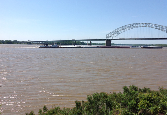
Hydraulically wide, with β = 5/3, for which the wetted perimeter P is a constant (Fig. 3), and Fns = 1.5;
Triangular, with
β = 4/3, for which the top width T is proportional to the flow depth d (Fig. 4), and Fns = 3; and
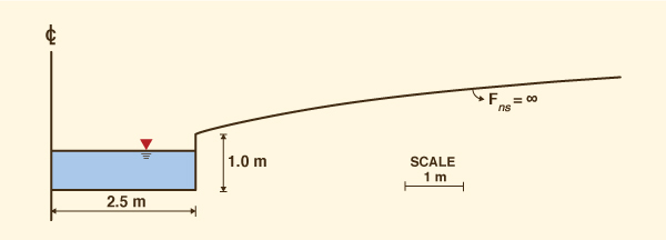
Inherently stable, with β = 1, for which the hydraulic radius R in the upper subsection [the overflow subsection] is constant and equal to that of the lower subsection (Fig. 5), and
Fns = ∞.
|
Fig. 3 Mississippi River at Mud Island, Memphis, Tennessee.
|
Fig. 4 The triangular channel cross-section.
|
Note that while, under Manning friction, the hydraulically wide channel becomes unstable at F = 1.5, and the triangular channel at F = 3,
the inherently stable channel becomes unstable as F ⇒ ∞.
The existence of a lower limit for boundary friction imposes a practical upper limit to the Froude number. To estimate this upper limit, we invoke
the dimensionless Chezy formula (Ponce, 2014d):
in which So = channel slope, and f = dimensionless friction factor, equal to 1/8 of the Darcy-Weisbach friction factor fD.
Assume a very steep slope (say, 45°, i.e., 100%), for which So = 1; and the lowest possible value of friction factor, f = 0.001875, corresponding to
a Darcy-Weisbach fD = 0.015. This assumption leads to an estimate of the maximum value of Froude number than can be achieved in practice: Fmax = 23 (Chow, 1959).
It is concluded that the inherently stable will never achieve
the asymptotic Froude number Fns = ∞ which characterizes it.
Therefore, constructing an inherently stable channel, for which β = 1, provides an unrealistically high factor of safety against roll waves.
This suggests the possibility of designing a practically stable cross-section, still one
where the risk of roll waves
would be so small as to be of no concern.
Assume a realistic maximum value of Froude number Fmax = 25. Using Eq. 8, at neutral stability, V = 1, and,
therefore, β = 1.04. It is concluded that a conditionally stable channel may be designed
to correspond to β = 1.04, and that there appears to be no need
to impose the asymptotic value of β = 1 in order to achieve hydrodynamic stability.
Thus, a channel designed with β = 1.04 is poised to provide
complete freedom from roll waves.
3. THE INHERENTLY STABLE CHANNEL
To derive the equation of the inherently stable channel, the general relation between wetted perimeter P and flow area A
is postulated in the following exponential form (Ponce and Porras, 1995d):
from which:
|
A dP dP
δ = ____ _____ = R _____
P dA dA
| (13) |
For the hydraulically wide channel, the wetted perimeter P is a constant (Section 2).
Therefore, from Eq. 12: δ = 0, and the
wetted perimeter remains:
|
P = Κo | [Hydraulically wide] |
| (14) |
and:
For the triangular channel, both the hydraulic radius R and the wetted perimeter P vary with the flow area,
and the exponent δ has the central value
δ = 0.5. From Eq. 12, the relation between hydraulic radius R, wetted perimeter P,
and flow area A is:
P = Κ A 0.5 [Triangular] |
| (16) |
and:
dP P
____ = 0.5 _____
dA A
| (17) |
For the inherently stable channel, the hydraulic radius R is a constant (Section 2). Therefore, from Eq. 12:
δ = 1, and the wetted perimeter remains:
P = Κo A [Inherently stable] |
|
(18) |
and:
dP P
____ = _____ = Κo
dA A
| (19) |
For the case of Manning friction, δ = 0 corresponds to β = 5/3, and δ = 1 corresponds to β = 1 (Section 2). Therefore,
the following linear relation holds:
5 2
β = ____ - ____ δ
3 3
| (20) |
Multiplying Eq. 20 by 3/2 and solving for δ:
5 3
δ = ____ - ____ β
2 2
| (21) |
Given a chosen value of neutral-stability Froude number Fns, Eq. 9 can be used to calculate β,
and Eq. 21 used to calculate δ.
Furthermore, assume that the optimum stable channel design is
that associated with Fns = 25,
for which βo = 1.04, and that the factor of safety for this case
is postulated to be F.S.i = 1.
For a given choice i of Fns,i, a factor of safety is defined as follows:
Table 1 shows selected values of parameters of the stable channel,
for suitable values of neutrally stable Froude numbers in the range
10 ≤ Fns ≤ ∞.
We conclude that a choice of Fns = 20
has a lesser chance of developing roll waves than a choice of Fns = 10.
Furthermore, a choice of Fns ≥ 25 is practically bound to assure
freedom from roll waves.
| Table 1. Selected parameters of the stable channel.
|
| Fns |
β |
δ |
Type |
F.S.i |
| 3 |
1.333 |
0.5 |
Conditionally stable |
0.78 |
| 5 |
1.20 |
0.700 |
Conditionally stable |
0.87 |
| 10 |
1.10 |
0.850 |
Conditionally stable |
0.95 |
| 20 |
1.05 |
0.925 |
Conditionally stable |
0.99 |
| 25 |
1.04 |
0.940 |
Strongly conditionally stable |
1.00 |
| 50 |
1.02 |
0.970 |
Strongly conditionally stable |
1.02 |
| 100 |
1.01 |
0.985 |
Strongly conditionally stable |
1.03 |
| 1000 |
1.001 |
0.9985 |
Quasi inherently stable |
1.04 |
| 5000 |
1.0002 |
0.9997 |
Quasi inherently stable |
1.04 |
| 10000 |
1.0001 |
0.99985 |
Quasi inherently stable |
1.04 |
| ∞ |
1.000 |
1.000 |
Inherently stable |
1.04 |
4. STABLE CHANNEL DESIGN
Liggett (1975) derived the differential equation of the inherently stable channel, for which δ = 1.
Ponce and Porras (1995d) extended this equation to
the conditionally stable channel, for which
δ < 1. Table 1 shows the values of β and
δ corresponding to selected values of Fns. The conditionally stable channel is stable, i.e., V ≤ 1,
provided the Froude number is restricted to F ≤ Fns, while the hydraulic radius varies
mildly with the flow depth.
Due to symmetry, a half-cross-section analysis is appropriate.
Hereafter, the asterisk (* ) is used as a subscript to refer to half values of the hydraulic variables, e.g.,
T* = half top width.
The differential wetted perimeter of the stable cross section is:
dP* =
[ (dh) 2 + (dT* ) 2 ] 1/2
| (23) |
in which dh = differential flow depth. Dividing by dh, and since dA* = T* dh (Ponce, 2014):
dP*
dT*
T* ______ =
[ 1 + ( ______ ) 2 ] 1/2
dA* dh
| (24) |
Substituting Eq. 13 into Eq. 24:
δ T*
dT*
______ =
[ 1 + ( ______ ) 2 ] 1/2
R dh
| (25) |
The inherently stable channel is that for which δ = 1; therefore, the hydraulics radius is constant and equal to Ro, i.e., Κo in Eq. 18.
Operating in Eq. 25, the differential equation of the inherently stable channel is obtained:
dT*
T*
______ =
[ ( _____ ) 2 - 1 ] 1/2
dh Ro
| (26) |
subject to T* > Ro .
Equation 26 may be solved using the following indefinite integral (Spiegel et al., 2013):
dx
∫ ______________ =
ln [ x + (x 2 - a 2) 1/2 ]
(x 2 - a 2) 1/2
| (27) |
in which x = T* , and a = Ro .
The design of a stable channel requires that the hydraulic radius be specified at the start.
To achieve this requirement, the cross section must be comprised of two subsections:
A lower subsection, of rectangular, trapezoidal, or triangular shape; and
An upper subsection, of stable shape (see, for instance, Fig. 5).
The lower subsection (of half bottom width B* , depth ho, and size slope z : 1 (H:V) defines the hydraulic radius Ro:
0.5 (2 B* + zho) ho
Ro =
________________________
B* + ho
(1 + z 2)1/2
| (28) |
In addition to defining Ro, the lower subsection serves the purpose of
conveying the low flows. In practice, high-velocity flows may occur at relatively small flow depths.
This fact should be taken into account in the design of the lower subsection.
Equation 26 constitutes a family of inherently stable channel cross sections, with parameter Ro. A particular solution, where
T*o
is the half top width corresponding to the depth
ho , is:
T* T*
______ + [ ( _____ ) 2 - 1 ] 1/2
Ro Ro
h = ho + Ro ln { _________________________________ }
T*o T*o
______ + [ ( _____ ) 2 - 1 ] 1/2
Ro Ro
| (29) |
For the special case of T*o = Ro ,
Eq. 29 reduces to the Liggett (1975)
solution for the inherently stable channel:
T* T*
h = ho + Ro ln {
______ + [ ( ______ ) 2 - 1 ] 1/2 }
Ro Ro
| (30) |
Since boundary friction has a lower limit and cannot realistically decrease to zero,
it follows that there is an upper limit to the Froude number that can be achieved in practice.
In other words, the inherently stable channel will become unstable
as the Froude number F ⇒ ∞, yet
the latter cannot be reached in any practical setting. Therefore, there appears to be no
need to design a stable channel section with δ = 1.
Alternatively, a channel section with a value δ < 1 may be designed to remain stable,
provided the neutrally stable Froude number associated with this value of δ
is not exceeded.
In practice, given that the maximum Froude number is not likely to exceed F = 25, a conditionally stable channel section,
for which δ = 0.94, may be envisaged.
Values of δ
corresponding to selected values of Fns are shown in Table 1.
The extension of Eq. 26 to the conditionally stable channel, for which δ < 1, is:
dT*
δT*
_____ =
[ ( ______ ) 2 - 1 ] 1/2
dh R
| (31) |
subject to δT* > R .
Unlike Eq. 26, Eq. 31 cannot be integrated analytically.
The shape of the upper subsection T* = f (δ, Ro, R ) may be obtained
by numerical integration, given a value of δ, corresponding to
a choice of Fns, and the hydraulic radius Ro corresponding to
the depth ho of the lower subsection.
The numerical integration proceeds by
selecting the shape of the lower subsection (B*,
ho, and z ) and the total channel depth ht , to comprise lower and upper subsections.
In the lower subsection, the flow depth varies in the range 0 ≤ h ≤ ho;
in the upper subsection, it varies in the range ho < h ≤ ht .
INPUT DATA
Half bottom width of the lower subsection B*
Depth ho of the lower subsection
Side slope of the lower subsection z
Relative
depth of the upper subsection hu' =
(ht - ho)/ho
Channel slope So Manning's n
Neutrally stable Froude number Fns
|
The computational algorithm is based on the following recursive procedure.
|
RECURSIVE PROCEDURE
With Fns ,
calculate β using Eq. 8.
With β,
calculate δ using Eq. 20.
Set counter i = 0
Calculate the half top width T*o
[at ho]: T*o = B* + zho
Calculate the half wetted perimeter P*o: P*o =
B* + ho (1 + z 2) 1/2
Calculate the half flow area A*o: A*o =
0.5 (2 B* + zho) ho
Calculate the hydraulic radius Ro: Ro =
A*o / P*o
Calculate the mean velocity Vo:
Vo = (1/n)
Ro 2/3 So1/2
Calculate the hydraulic depth Do:
Do = A*o / T*o
Calculate the Froude number Fo:
Fo = Vo /
(g Do )1/2
Calculate the half discharge Q*o:
Q*o = Vo
A*o
Set Δh = 0.0001 m
⇐ ⇐ ⇐ ⇐ ⇐ ⇐
⇓
Increment the counter i by 1
Calculate the flow depth hi :
hi = hi - 1 + Δh
Using Eq. 29, calculate the increment ΔT*i :
ΔT*i = Δh
[ (δ T*i - 1 / R*i - 1 ) 2 - 1 ] 1/2
Calculate the increment ΔP*i :
ΔP*i = [ (Δh)2 + (ΔT*i )2 ] 1/2
Calculate the increment ΔA*i :
ΔA*i = 0.5 ( 2T*i - 1 + ΔT*i ) Δh
Calculate the value of T*i [at hi ]:
T*i
= T*i - 1
+ ΔT*i
Calculate the value of P*i :
P*i
= P*i - 1
+ ΔP*i
Calculate the value of A*i :
A*i
= A*i -1
+ ΔA*i
Calculate the value of Ri :
Ri
= A*i / P*i
Calculate the mean velocity Vi :
Vi = (1/n)
Ri 2/3 So1/2
Calculate the hydraulic depth Di :
Di = A*i / T*i
Calculate the Froude number Fi :
Fi = Vi /
(g Di )1/2
Calculate the discharge Q*i
corresponding to the flow depth hi :
Q*i = (1/n) A*i
R*i 2/3 So1/2
Return to Step 13,
and proceed recursively, until hi ≥ ht .
⇑
⇐ ⇐ ⇐ ⇐ ⇐ ⇐
|
5. ONLINE CALCULATOR
The calculator ONLINE INHERENTLY STABLE solves the recursive algorithm explained in the previous section.
Input data to
the calculator consists of: Geometric and hydraulic data:
half bottom width B* , depth ho , side slope z ,
relative depth hu' , channel slope So, and Manning's n;
and Neutrally stable Froude number Fns.
To solve for the inherently stable channel, specify a very high value of neutrally stable Froude number, say Fns = 10,000.
To solve for the conditionally stable channel, specify a realistically high value of neutrally stable Froude number, say Fns = 25 (Section 2).
6. ANALYSIS
Table 2 shows
a summary of typical results of calculations of the stable channel. The following data set was used for the example shown in Table 2:
|
EXAMPLE INPUT DATA
Half bottom width B* = 2.5 m
Depth ho = 1 m
Side slope z = 0
Relative depth hu' = 1
Channel slope So = 0.012
Manning's n = 0.015
Neutrally stable Froude number: Ten (10) values,
varying in the range: 3 ≤
Fns ≤ 10,000
|
For increased accuracy, the depth interval is set at Δh = 0.0001 m.
In this example, the results of the
recursive computation are printed once every 1000 increments, i.e.,
the depth interval for output is Δhout = 0.1 m.
As expected, Table 2 shows that the hydraulic radius for Fns = 10,000
remains
practically constant and equal to R = 0.714 m throughout the indicated range of flow
depths in the upper subsection (1 ≤ h ≤ 2).
The examination of Table 2,
supplemented with results obtained using ONLINE INHERENTLY STABLE lead to the following conclusions:
For h > ho, the smaller the choice of Fns, the smaller
the resulting stable top width.
For h > ho, the larger the choice of Ro, the smaller
the resulting stable top width.
Given
Fns, the larger the choice of Ro, the narrower
the resulting stable channel section.
Given
Ro, the smaller the choice of Fns, the narrower
the resulting stable channel section.
These results confirm and extend the findings of Ponce and Porras (1995e).
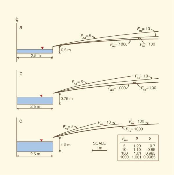
Fig. 6 Stable channel cross sections as a function of neutrally stable Froude number Fns and
hydraulic radius Ro:
(a) ho = 0.5 m, Ro = 0.417 m;
(b) ho = 0.75 m, Ro = 0.577 m; and
(c) ho = 1.0 m, Ro = 0.714 m
(redrawn from Ponce and Porras, 1995e).
A comparison of the inherently stable
or conditionally stable
channels with a rectangular channel of the same bottom width,
channel slope and boundary roughness,
shows that for both channels the discharge and Froude number are likely to vary
gradually with stage, with the latter either increasing or decreasing, depending on the flow conditions.
Theory, however, predicts that while the inherently stable channel will always
remain stable, and the conditionally stable channel will most likely remain stable throughout
a practical range of Froude numbers, the rectangular channel
may be poised to
eventually develop roll or pulsating waves.
7. DESIGN EXAMPLE
Design a stable channel for the following data: baseflow Qb = 10 m3/s, peak flow Qp = 100 m3/s, half bottom width B* = 2.5 m, size slope z = 0,
channel slope So = 0.012, and Manning's n = 0.015.
Calculate the depth ho and relative depth hu'.
Solution.
Trial runs with lower subsection depth ho = 0.8 m, and
ratio of upper-to-lower subsection depths hu' = 2.0, show the following results:
For the inherently stable channel, at
Fns = 10,000: Lower subsection discharge
Qb = 10.46 m3/s, and
total discharge, corresponding
to a total channel depth
ht =
ho (hu' + 1) = 2.4 m,
is
Qp = 112.112 m3/s.
The hydraulic radius remains Ro =
0.606 m through the range 0.8 ≤ ht ≤ 2.4, and the half top width T* at ht = 2.4 m is: T* = 34.468 m.
For the conditionally stable channel, at Fns = 25: Qb = 10.46 m3/s, and Qp = 102.902 m3/s. At ht = 2.4 m, the
hydraulic radius is R =
0.692 m and the half top width is: T* = 25.169 m.
In this example, the design half top width of the conditionally stable channel
is equal to 73% of that of the inherently stable channel, i.e., a reduction of 27% is indicated.
8. CONCLUSIONS
The inherently stable channel and its conditionally stable
alternative are reviewed, elucidated, and
calculated online.
The asymptotic neutrally stable Froude number for the inherently stable channel
is Fns ⇒ ∞.
Theoretically, such a channel will become neutrally stable when the Froude number reaches infinity.
Since the latter is a physical impossibility,
this requirement effectively guarantees that
the inherently stable channel will always remain well
below the threshold of instability, regardless of flow discharge,
thus completely eliminating the possibility of roll wave formation.
The inherently stable channel will never achieve
the value of Froude number Fns = ∞ which characterizes it.
Therefore, constructing an inherently stable channel, i.e., that
for which the exponents β = 1 and δ = 1, provides an unrealistically high factor of safety against roll waves.
This suggests the possibility of designing instead a conditionally stable cross-sectional shape, for a suitably high but realistic
Froude number such as Fns = 25, corresponding to
β = 1.04 and δ = 0.94,
for which the risk of roll waves
would be so small as to be of no practical concern.
The results of this study
lead to the following conclusions:
For h > ho, the smaller the choice of Froude number Fns, the smaller
the resulting stable top width.
For h > ho, the larger the choice of hydraulic radius Ro, the smaller
the resulting stable top width.
Given
Fns, the larger the choice of Ro, the narrower
the resulting stable channel section.
Given
Ro, the smaller the choice of Fns, the narrower
the resulting stable channel section.
A design example shows that the conditionally stable
channel with Fns = 25 is about 27% narrower than the
inherently stable channel.
REFERENCES
Chow, V. T. 1959. Open-channel hydraulics. McGraw-Hill, New York.
Cornish, V. 1907. Progressive waves in rivers. The Geographical Journal, Vol. 29, No. 1, January, 23-31.
Craya, A. 1952. The criterion for the possibility of roll-wave formation. Gravity Waves, Circular 521,
National Bureau of Standards, Washington, D.C., 141-151.
Lagrange, J.-L., 1788. "Mémoire sur la Théorie du Mouvement des Fluides," Bulletin de la Classe des Sciences Academie Royal de Belique, No. 1783, pp. 151-198.
Liggett, J. A. 1975. Stable Channel Design, in Chapter 6: Stability,
in Unsteady Flow in Open Channels, K. Mahmood and V. Yevjevich, editors, Water Resources Publications, Fort Collins, Colorado.
Lighthill, M. J., and G. B. Whitham. 1955. On kinematic waves: I. Flood movement in long rivers. Proceedings, Royal Society of London, Series A, 229, 281-316.
Molina, J., J. Marangani, P. Ribstein, J. Bourges, J.-L. Guyot, and C. Dietz. 1995.
Olas pulsantes en ríos canalizados de la región de La Paz. Bull. Inst. fr. études andines, Vol. 24, No. 3, 403-414.
Montuori, C. 1965. Spontaneous formation of wave trains in channels with a very steep slope.
Synthesis of theoretical research and interpretation of experimental results,
Translation No. 65-12, U.S. Army Engineer Waterways Experiment Station, Corps of Engineers, Vicksburg, Mississippi, August, 44 p.
Ponce, V. M., and D. B. Simons. 1977. Shallow wave propagation in open channel flow.
Journal of the Hydraulics Division, ASCE, Vol. 103, No. HY12, December, 1461-1476.
Ponce, V. M. 1992. Kinematic wave modelling: Where do we go from here?
International Symposium on Hydrology of Mountainous Areas,, Shimla, India,
May 28-30, 485-495.
Ponce, V. M. 1991. New perspective on the Vedernikov number.
Water Resources Research, Vol. 27, No. 7, July, 1777-1779.
Ponce, V. M., and M. P. Maisner. 1993. Verification of theory of roll-wave formation.
Journal of Hydraulic Engineering, ASCE, Vol. 109, No. 6,
June, 768-773.
Ponce, V. M., and P. J. Porras. 1995. Effect of cross-sectional shape on free-surface instability. Journal of Hydraulic Engineering, ASCE, Vol. 121, No. 4,
April, 376-380.
Ponce, V. M. 2014. Fundamentals of open-channel hydraulics.
Online text.
Powell, R. W. 1948. Vedernikov's criterion for ultra-rapid flow.
Transactions, American Geophysical Union, Vol. 29, No. 6, 882-886.
Seddon, J. A. 1900. River hydraulics. Transactions, ASCE, Vol. XLIII, 179-243, June.
Spiegel, M. R., S. Lipschutz, and J. Liu. 2013. Mathematical handbook of formulas and tables. Fourth Edition, Schaum's Outline Series. McGraw Hill, New York, p. 80.
Vedernikov, V. V. 1945. Conditions at the front of a translation wave disturbing a
steady motion of a real fluid. Comptes Rendus (Doklady) de l' Académie des Sciences de l' U.R.S.S., Vol. 48, No. 4, 239-242.
Vedernikov, V. V. 1946. Characteristic features of a liquid flow in an open channel. Comptes Rendus (Doklady) de l' Académie des Sciences de l' U.R.S.S., Vol. 52, No. 3, 207-210.
|